Getting started

This notebook is executed on every docs build — if it stops running against the latest complextorch, CI fails. Treat it as a smoke-test of the public API as well as a tutorial.

1 · Imports & version check

import torch
import complextorch as ctorch

print(f"torch        {torch.__version__}")
print(f"complextorch {ctorch.__version__}")

torch        2.11.0+cu130
complextorch 2.0.0

2 · Building a complex tensor

complextorch operates on complex-dtype torch.Tensor (typically torch.cfloat). There is no special wrapper type — use PyTorch’s built-ins directly:

torch.manual_seed(0)

x = torch.randn(8, 5, 16, dtype=torch.cfloat)   # (batch, channels, length)
print(x.shape, x.dtype)
print(x[0, 0, :3])

torch.Size([8, 5, 16]) torch.complex64
tensor([-0.7961-0.8148j, -0.1772-0.3068j,  0.6001+0.4893j])

You can construct from magnitude / phase via torch.polar:

mag   = torch.rand(8, 5, 16)
phase = torch.rand(8, 5, 16) * (2 * torch.pi) - torch.pi
z = torch.polar(mag, phase)
print(z.dtype, z[0, 0, 0])

torch.complex64 tensor(0.0721-0.1039j)

3 · Conv1d + Linear (the README example)

The native cfloat modules (Conv1d, Linear, …) are thin wrappers around torch.nn with dtype=torch.cfloat. See Native vs. Gauss-trick modules for the design rationale.

conv = ctorch.nn.Conv1d(in_channels=5, out_channels=16, kernel_size=3)
fc   = ctorch.nn.Linear(in_features=16 * 14, out_features=4)

h = conv(x)                       # (8, 16, 14)
h_flat = h.reshape(h.size(0), -1) # (8, 16*14)
y = fc(h_flat)                    # (8, 4)

print("conv output:", h.shape, h.dtype)
print("fc output:  ", y.shape, y.dtype)

conv output: torch.Size([8, 16, 14]) torch.complex64
fc output:   torch.Size([8, 4]) torch.complex64

Both modules accept and emit complex tensors — and gradients flow through them just like any real-valued torch.nn module:

loss = y.abs().pow(2).mean()
loss.backward()

total_grad_norm = sum(p.grad.abs().pow(2).sum() for p in conv.parameters()).sqrt()
print(f"loss = {loss.item():.4f}, conv grad norm = {total_grad_norm:.4f}")

loss = 0.4308, conv grad norm = 0.9106

4 · Type-A vs. Type-B activations

The package implements two paradigms for complex activations (see Activations for the math). Let’s compare a Type-A CVSplitReLU (independent real/imag) against a Type-B modReLU (magnitude-only) on the same input.

import matplotlib.pyplot as plt

z = torch.complex(
    real=torch.linspace(-2, 2, 200).repeat(200, 1),
    imag=torch.linspace(-2, 2, 200).repeat(200, 1).T,
)

split_relu = ctorch.nn.CVSplitReLU()
mod_relu   = ctorch.nn.modReLU(bias=-0.5)

with torch.no_grad():
    a = split_relu(z)
    b = mod_relu(z)

fig, axes = plt.subplots(2, 2, figsize=(8, 7), sharex=True, sharey=True)
for ax, data, title in zip(
    axes.flat,
    [a.abs(), a.angle(), b.abs(), b.angle()],
    ["CVSplitReLU |·|", "CVSplitReLU ∠", "modReLU |·|", "modReLU ∠"],
):
    im = ax.imshow(data, extent=[-2, 2, -2, 2], origin="lower",
                   cmap="twilight" if "∠" in title else "viridis")
    ax.set_title(title)
    fig.colorbar(im, ax=ax, fraction=0.046, pad=0.04)
axes[1, 0].set_xlabel("Re(z)"); axes[1, 1].set_xlabel("Re(z)")
axes[0, 0].set_ylabel("Im(z)"); axes[1, 0].set_ylabel("Im(z)")
plt.tight_layout();

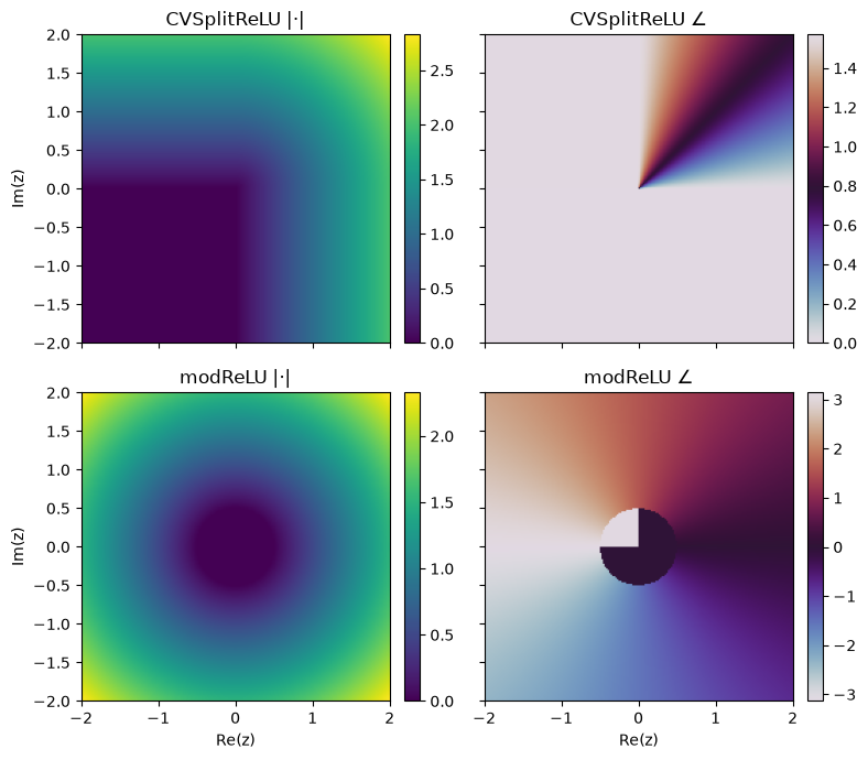
CVSplitReLU zeros the real/imag components independently — it doesn’t preserve phase. modReLU only modulates magnitude (|z| - b)+ and leaves the phase untouched.

5 · Welch’s PSD on a complex signal

complextorch.signal.pwelch() is a torch port of scipy.signal.welch that’s differentiable end-to-end — so it can sit inside a loss function.

from complextorch.signal import pwelch

t = torch.linspace(0, 1, 4096)
sig = torch.exp(1j * 2 * torch.pi * 50 * t).to(torch.cfloat) \
    + 0.5 * torch.exp(1j * 2 * torch.pi * 120 * t).to(torch.cfloat) \
    + 0.1 * torch.randn(4096, dtype=torch.cfloat)

f, psd = pwelch(sig, fs=4096.0, window=256, n_overlap=128)

plt.figure(figsize=(7, 3))
plt.semilogy(f.numpy(), psd.numpy())
plt.xlabel("Frequency (Hz)"); plt.ylabel("PSD"); plt.title("pwelch demo")
plt.tight_layout();

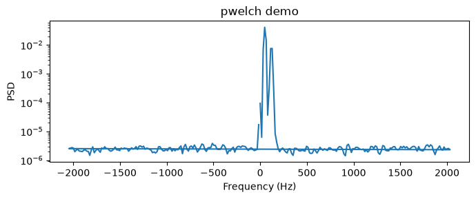
The two tones at 50 Hz and 120 Hz should be clearly visible. Because pwelch is autograd-friendly, you can use the PSD as a spectral loss for training a complex-valued generator network.

Where next?

• Browse the API reference for the full module surface (nn, signal, transforms, datasets, models).

• Read the Activations deep-dive for Type-A / Type-B / fully-complex / ReLU-variant theory.

• Check the changelog for what landed in the current release.